We refer to the case study of Sicily (Fig. 1), one of the 20 regions of Italy. We have retrieved hourly rainfall from 306 rain gauges distributed within the region, managed by the regional water observatory (Osservatorio delle Acque, OdA), the SIAS (Sicilian Agro-meteorological Information Service), and the Regional Civil Protection Department (DRPC). Figure 1 shows the rain gauge locations for the period January 2009–October 2018 (green dots) and those available only for the period January 2014–October 2018 (black dots).

Landslide data are retrieved from the FraneItalia database compiled by Calvello and Pecoraro (2018) (see locations in Fig. 1). This database contains information on landslides that occurred in Italy from January 2010 to December 2019 and is available online (https://franeitalia.wordpress.com/database/, last access: 17 November 2021). Thus, our analysis is based on the period from January 2010 to October 2018, where both rainfall and landslide information is available. Some landslide events have been removed from the analysis. In particular, this was done based on the landslide typology, material, and type of trigger. Only events having a “rainfall” or “rainfall and other” trigger have been considered so as to exclude landslides due to earthquakes and anthropogenic activities. Rockfalls have been removed from the analysis as well as their triggering cannot always be linked to rainfall. Rainfall data have been checked in order to remove suspicious rainfall data. In particular, where hourly rainfall exceeded 250 mm – corresponding to about one-third of mean yearly rainfall for Sicily and to about 2 times the maximum rainfall ever recorded in 1 h – the series has been visually inspected, and in the case of an evident error (rain gauge malfunction) the whole rainfall event surrounding the peak has been removed. In light of the above, a flow chart representing the applied methodology is shown in Fig. 2a.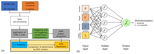

Figure 2Flow chart illustrating the methodology (a) and the artificial neural network architecture considered (b).

Download

First, pre-processed precipitation and landslide data were inputted to the CTRL-T (Calculation of Thresholds for Rainfall-induced Landslides-Tool) code (Melillo et al., 2018). The software consists of a code in the R language and allows rainfall events to be reconstructed and characterised by the following variables: duration D, mean intensity I, total depth E=D×I, and peak intensity Ip (defined as the maximum hourly intensity occurring during a rainfall event). The most probable rainfall conditions associated with each landslide event (multiple rain gauges available for a given location) are computed by the software based on distance between the rain gauge and the landslide location as well as the characteristics of the reconstructed rainfall event. In particular, for a given landslide, all rain gauges within a circle of radius Rb specified by the user are searched, and, when more than one rain gauge is located within the circle, the rainfall events from each rain gauge are weighted based on the rain gauge–landslide distance and the rainfall event characteristics (cumulated rainfall and duration). The weight is used to estimate the “probability” associated with each rainfall condition potentially attributable to each landslide event. In particular, the probability, in the case of multiple rainfall conditions, is computed by dividing each weight by the sum. CTRL-T then determines the triggering rainfall conditions of each landslide as those corresponding to the highest probability. Finally, the code provides power law E–D thresholds for different levels of non-exceedance frequency of triggering events. The software allows the user to set different values of the parameters to reconstruct rainfall events in order to take into account seasonality, i.e. different average evapotranspiration rates in different periods of the year. Specifically, following the study by Melillo et al. (2016), we assumed that in the warm season CW (April–October) the minimum dry period separating two rainfall events is P4warm=48 h, while in the cold season a longer period is assumed (P4cold=96 h). The rain gauge sensitivity is Gs=0.1 mm. The rain gauge search radius has been fixed to Rb=16 km. A binary coding has been attributed to each rainfall event, flagging triggering events as a target with a value of 1 and a non-triggering event with a null value. Application of the CTRL-T software allowed the rainfall events associated with the 144 landslide events in the inventory (triggering events) and 47 398 non-triggering events to be reconstructed. For 103 events, only the day of triggering was known, while for the remainder a more precise indication of the triggering instant was available. In the first case, the triggering instant was attributed to the end of the day, in the second case to the instant of peak rainfall within the time interval when the triggering occurred. Furthermore, for the 144 landslide events, detailed information on the typology was available only in 18 cases, 10 of which were “fall of more than one material”, 4 were “flow”, and the remaining 4 were “slide”. The average distance between the rain gauge and landslide for the 144 events is about 5 km; thus the maximum value of Rb=16 km was seldom reached.

Table 1Results of tests with ANNs, showing the optimal number of hidden neurons (a number from 5 to 20 has been tested) and the true skill statistics (TSSs) for the entire, the training, the validation, and the test data sets. Values in the table are compared to TSS0=0.50, which is the maximum value associated with a D–E power law threshold.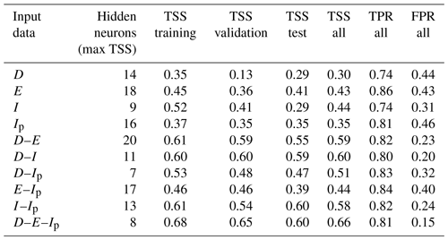

Download Print Version | Download XLSX

The characteristics of the events were used as input variables to ANNs devised for pattern recognition, as implemented within the neural net pattern recognition tool in MATLAB®. The neural network, characterised by a feed-forward structure, is composed of three layers: input, hidden, and output (Fig. 2b). The input layer takes the series of predictors and sends them to the hidden layer, where the series are combined and transformed though a specific activation function. Two different activation functions have been considered – a tan-sigmoid function f(n) for the hidden layer and a log-sigmoid g(n) for the output layer:

The ANNs have been trained through the scaled conjugate gradient backpropagation algorithm, while cross-entropy was assumed to be the performance function for training. Denoting the generic ANN output with yi (assuming values in the open interval between 0 and 1) and the binary target with ti, i=1, 2, …, N, the cross-entropy function F heavily penalises inaccurate predictions and assigns minimum penalties for correct predictions:

The ability to distinguish triggering events from non-triggering events was measured using the confusion matrix, a double-entry table in which it is possible to identify true positives (TPs; triggering events correctly classified), true negatives (TNs; non-triggering events correctly classified), false negatives (FNs; triggering events classified as non-triggering), and false positives (FPs; non-triggering events classified as triggering). Through the confusion matrix it is possible to determine the true positive rate (TPR) and the false positive rate (FPR) as well as their difference, known as the true skill statistic (TSS), which is widely used for threshold determination (Peres and Cancelliere, 2021):

The output of the ANNs is transformed into a binary code (dichotomisation) by assuming a value of 1 (ANN predicts a landslide) when the output is greater than a threshold value and a value of 0 otherwise. We then identify the mentioned threshold value by maximising the TSS, which has the advantage of not being affected by unbalanced training data set issues with respect to other indices, such as accuracy ACC = (TP + TN)/(TP + TN + FP + FN) – a performance metric used as default by many ANN training software tools. Maximisation of TSS implicitly assumes that all entries of the confusion matrix have the same utility. Quantifying the loss of a false negative with respect to a false positive is a complex task that goes beyond the aim of the present analysis and that has been faced only in very recent studies (cf. Sala et al., 2021). Results from ANNs are compared with rainfall duration–depth power law thresholds derived through the maximisation of TSS, i.e. again, analysing both triggering and non-triggering events.

For our analysis different combinations of input data (duration D, intensity I, total depth E, and peak intensity Ip) and different architectures, changing the number of hidden neurons, were tested. In particular, the following input variable configurations have been investigated: (1) D; (2) E; (3) I; (4) Ip; (5) D and E; (6) D and I; (7) D and Ip; (8) E and Ip; (9) I and Ip; (10) D, E, and Ip. The listed input configurations are indeed all possible ones, except those combining both E and I with duration D. This has been done because the two pairs D–I and D–E have the same informative content by construction, as confirmed by the fact that the performances of the D–I and D–E neural networks do not differ significantly (see Table 1); slight differences may occur as ANNs can be sensitive to how a set of variables with the same information content as another are presented to the network. All the data have been inputted taking their natural logarithms. Different networks have been considered, varying the number of hidden neurons from 5 to 20, in order to search for the best value, i.e. the one yielding the highest TSS.

The entire data set of rainfall events was divided into a training, a validation, and a test data set, selected randomly from the entire data set, in the proportions of 70 %, 15 %, and 15 %. The training data set is data used to fit the model, while the validation provides an unbiased evaluation of a model fit on the training data set while tuning model hyperparameters, such as the number of training iterations. Finally, the test data set provides an unbiased evaluation of a final model fit. This subdivision allowed the early-stopping criterion to be applied to prevent overfitting. According to this criterion, the training of the neural network is stopped when the values of the performance function calculated on the validation data set start to get worse. In order to ensure representativeness of the data randomly assigned to the training, validation, and test data sets, results where the TSS in the test or the validation data set are greater than the TSS in the training data set are removed from the analysis. Once the network is developed considering these three data sets and early stopping, it is “frozen”, and metrics from the confusion matrix (e.g. TSS) can be computed with that network on the entire data set, and the corresponding performances can be considered generalisable. Thus, when comparing our proposed approach with the traditional one, we focus on these last performances (labelled “all”). This seems to be the most appropriate way to proceed as the I–D power law and its performance are determined with respect to the entire data set.